Using FT8 to Benchmark Station Rx Performance with wsjt_all
Introduction
This page gives some background about why I developed wsjt_all; a bit about my personal exploration of ways to check that I'm getting the best possible performance out of my ham radio station, given the constraints I have. Every ham radio station has constraints of *some* kind, and part of the fun of the hobby for me is working out how to do the best with the situation you're in. Getting instant signal reports in volume from pskreporter has been a huge help in achieving this.My station
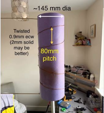
I live in a conservation area where no outside antennas are permitted, so everything I use is indoors. Some of the antennas that I use are inside the decorative glass fibre chimney shown below!
Despite this, when I look at pskreporter,
I often have the longest distance reach, and largest coverage area, of stations operating from my country (England), on what I would call
some of the most difficult bands; 80m, 160m, and 2m. And that's on both transmit and receive with a single Icom IC-7100 as the station transceiver.
I'm not claiming to 'win' all the time; clearly there are many stations with long Yagis reaching far into Europe on 2m and stations with superb
receiving antennas in remote locations who do far better than I do. But what I do know is that I'm winning the battle against local QRM and using
antennas that work well on transmit too, and I'm *absolutely* doing better than at least half of other stations irrespective of location.
Some of the antennas that I use are inside the decorative glass fibre chimney shown below!
Despite this, when I look at pskreporter,
I often have the longest distance reach, and largest coverage area, of stations operating from my country (England), on what I would call
some of the most difficult bands; 80m, 160m, and 2m. And that's on both transmit and receive with a single Icom IC-7100 as the station transceiver.
I'm not claiming to 'win' all the time; clearly there are many stations with long Yagis reaching far into Europe on 2m and stations with superb
receiving antennas in remote locations who do far better than I do. But what I do know is that I'm winning the battle against local QRM and using
antennas that work well on transmit too, and I'm *absolutely* doing better than at least half of other stations irrespective of location.
TL;DR - the antennas
 I've worked with attic antennas in two houses now over the last decade, and found that it's pretty easy to set up a fan dipole to cover at
least 20m to 10m if not 40m to 6m.
I've worked with attic antennas in two houses now over the last decade, and found that it's pretty easy to set up a fan dipole to cover at
least 20m to 10m if not 40m to 6m.
What I use currently is:
- 160, 80, 60, 40: Small transmitting loop 7.5m circumference made from 10mm copper tube
- 20, 15, 17, 10, 6m: fan dipole (I don't have 30m and 12m currently)
- 2m - my G1OJS Contraspiral (pictured right)
The thing that has made the most difference though is the addition of an active receive loop to these antennas for HF work. I use an LZ1AQ amplifier with a small loop made from 20mm wide aluminium strip, right at the top of the attic. Using the fan dipoles for Rx results in a very high noise floor even with careful minimisation (and measurement of) common mode currents. I have previously used an end-fed wire cut to 20m length, bent into a U shape to fit in my 5m x 5m attic space, which was great on transmit but even worse on receive than the fan dipoles as you would expect!
Benchmarking
After I had played the game of watching the noise level on the S meter whilst adding chokes, turning off ring mains and devices etc, running up and downstairs and scribbling notes and thinking "was that better?", I got interested in what I could do with pskreporter. Using the online maps helped me get a feel for how well my antennas were working on transmit, but I didn't get much info for receive. When I later learned that once you get a spot on pskrepoter from a particular station, you won't get another for at least 20 minutes, I started to dig into using the live data feed from mqtt.pskreporter.info where there is no 20 minute limitation on repeated spots.BandOpticon
The first thing I did with the live data feed was write some software to show a live view of the digi-mode activity to and from my neighboring ham stations (in nearby Maidenhead squares). This told me what band activity was like *now* and at least I could then tell if bands were active but for some reason I couldn't hear activity. That was the first objective measure in a sea of subjective ones! After a lot of work learning Python (where BandOpticon started) and then re-learning JavaScript, I developed BandOpticon into a web-based page so that anyone can use it. The current version is here. You can use this web page to see what bands are active, and get a view of what the connectivity is between your local squares or stations and remote squares/callsigns. There are some experimental views in there that look towards benchmarking too.Wsjt-all
After playing with the experimental views in BandOpticon, I started thinking about using the data in the WSJT-X 'all.txt' file. On a few occaions I had tried setting up a second instance of WSJT-X to make decodes using the audio from a web SDR, and watching the waterfalls to compare noise levels. I also tried copy and paste of the decodes from WSJT-X and went through them manually in notepad, matching up decodes to compare the reports. This provides some snapshot information, but is quite tedious to do repeatedly!But the 'all.txt' file records every decode made on receive, and I started thinking about using that as the data source. One problem here is that these files can become huge, and take an age to open in notepad (I eventually found Notepad++ which opens them much faster). So I started thinking about automating the process.
Wsjt_all, at Version 1.3, is focussed on exactly this problem. It takes two 'all.txt' files and looks for 'sessions' within them. I've defined a session as a set of decodes where the gap between one decode and the next doesn't exceed a particular number of seconds and the band and mode don't change. This alone is a useful thing to start with, and I made it the first step so that later versions might do something useful with indivudual all.txt files as well as pairs.
Once the sessions are found, the program looks for sessions that exist in both files at the same time (i.e. overlap in time to contain at least some decodes in each file). Once these sessions are found, they are processed to do some analysis based on the reports they contain.
Comparing SNR and just ... counting
At this point, I'm still searching for good ways to analyse and present the data.Comparing 'signal reports' automatically seems to be a good idea, and there is certainly some useful information there. However, this can only reasonably be done if the reports are simultaneous, or very close in time; if there is too much time between the reports, uncertainty creeps in due to fading and lack of knowledge about the transmitting station's power settings and beam heading (for example). And that also throws away the information about the callsigns received by one station and not the other.
Perhaps what's more important is the simple fact of whether a station was received or not - after all, that's the defining characteristic of communication. So counting the number of times each callsign was received in each all.txt file probably carries a lot of weight.
Wsjt_all Plots (V1.3)
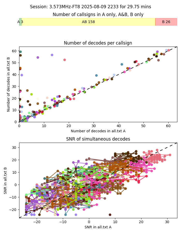
So, V1.3 produces plots like the one shown on the left.
At the top of the image, the title identifies the 'joint' session frequency, mode, start time and duration. Immediately under the title is a graphic that illustrates the number of callsigns received in A only, B only, and in both A and B. This alone is good information!
Below that, the first graph shows a coloured spot for each callsign received, with the X and Y axis showing the number of times that particular callsign was received in each all file. Points lying on the dashed diagonal line were received an equal number of times in each file (receive configuration). Points lying on one axis were received only in the all file referred to in the axis label. Note that some random movement is applied to the points so that points don't fully lie on top of each other, so points won't necessarily lie on an exact grid.
The second plot compares the SNR reports, only for callsigns with decodes in both all files. Again, points lying on the dashed diagonal line represent equality between each file (receive configuration). The number of callsigns received in a typical session on a very active HF band can easily be in the hundreds, and it is not possible to create a colour palette that enables the human eye to track individual callsigns in the mix. Hence, I've added lines connecting reports for each individual callsign. Note that this chart is not intended to be used for detailed inspection: it is the overall 'impression' that is important, along with 'outliers' that can be easily seen.
Next steps
Wsjt_all is quite new (I only started working on it about a week ago) and at the outset I didn't really know if the data could be displayed in a meaningful and useful way, let alone how to present it with the best clarity and information content.So one of the next things I'll do is experiment more with the plots. I might also add a 'data dump' feature for the chart data, so that others can produce their own plots. I've started tracking ideas in the 'issues' section on GitHub, so have a look there too.