Converting Bridge Voltages to Load Impedance: Method 3

Introduction

Calculating the complex load impedance from the quantities measured by a scalar network analyser or RF bridge, i.e. the magnitude of the impedance $\vert Z_L \vert$ and the magnitude of the complex reflection coefficient $\vert \Gamma \vert$ , requires quite a bit of algebraic manipulation if done from scratch. The accademic level required is roughly that at which people learn about quadratic equations, but it is easy to drop a minus sign or lose track of the route to the solution. This page presents a graphical / geometric approach, which might be easier to follow.

The Geometry

Magnitude of the Load Impedance

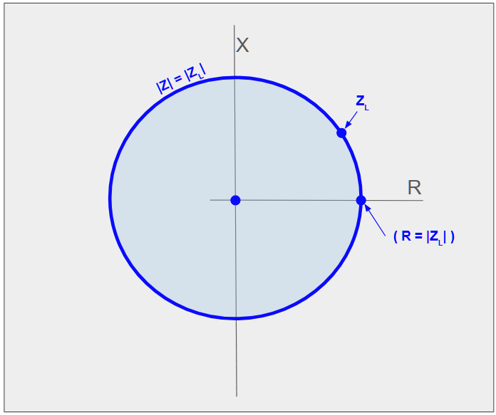
Firstly, we set up the problem by plotting an unknown load impedance $Z_L$ on the complex impedance plane, see diagram below. We can easily add a circle that captures all impedance values that have the same magnitude $\vert Z \vert$ as our unknown load. This circle crosses the real, or resistance, axis where $R = \vert Z_L \vert$, although we don’t need to remember this value for the steps that follow.

Magnitude of the Reflection Coefficient

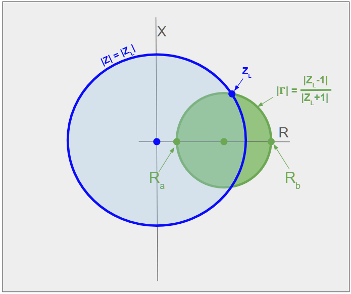
Next, let’s add a circle capturing all points that have the same magnitude of reflection coefficient, $\vert \Gamma \vert$, as our load. This circle clearly cuts through the point representing our load, but what other points? How do we find the unique circle that we need? The answer is quite straightforward; we know that it must cross the resistance axis at the place where a purely resistive load results in the the same magnitude of reflection coefficient, or same VSWR, as our load. There are two places where this occurs. These are, if we write VSWR as S: $R_a = Z_0/S$ and $R_b = Z_0S $ . These resistances are in inverse, or reciprocal, proportion to each-other. So, we can add a circle cutting through our load impedance and the two resistance values with the same VSWR.

Recall that, in units of normalised impedance,

$$S = \frac{1+\vert \Gamma \vert}{1-\vert \Gamma \vert} $$

So we can write our two resistances $R_a$ and $R_b$ in terms of our measured $\vert \Gamma \vert$:

$$R_a = \frac{1}{S} = \frac{1-\vert \Gamma \vert}{1+\vert \Gamma \vert} $$ and $$R_b=S=\frac{1+\vert \Gamma \vert}{1-\vert \Gamma \vert}$$

Three Distances

Now, we know the distance from the origin to our load impedance is $\vert Z_L \vert$, and we also now know that the distance from the origin to the centre of the $\vert \Gamma \vert$ circle is $\frac{R_a+R_b}{2}$, and the distance from there to the load impedance is simply the radius of the $\vert \Gamma \vert$ circle, which is $\frac{R_b-R_a}{2}$. So we have the lengths of all three sides of a triangle:

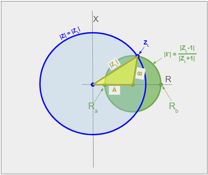
Now, the area of this triangle is related to the reactance of the load, because $X_L$ is simply the height of the triangle using side $A$ as the base:

\[area=\frac{1}{2}AX_L\]

We can also find the area of this triangle from the three known side lengths using Heron’s formula. One way to write this formula is:

\[area = \frac{1}{4}\sqrt{(a+b+c)(b+c-a)(a+c-b)(a+b-c)}\]

Whare a,b and c are the three lengths of the triangle’s sides.

So we can use the triangle’s area to link mod(Z) and mod(Gamma) to our load reactance. Let’s substitute our known lengths for a,b,c, and get rid of the square root by squaring both expressions for area above to get:

$$\frac{1}{4}A^2X_L^2 = \frac{1}{16}(A+B+\vert Z_L \vert)(B-A+\vert Z_L \vert)(A-B+\vert Z_L \vert)(A+B-\vert Z_L \vert) $$

so

$$X_L^2 = \frac{1}{4A^2}(A+B+\vert Z_L \vert)(B-A+\vert Z_L \vert)(A-B+\vert Z_L \vert)(A+B-\vert Z_L \vert) $$

Final Steps

Looking back to the diagram showing the triangle and the circles, we can easily see that $A+B$ is $R_b$, and $A-B$ is $R_a$, and we’ve already noticed that $R_b$ is the VSWR and $R_a$ is $\frac{1}{VSWR}$, so, writing VSWR as S and $\vert$ $Z_L$ $\vert$ as Z :

\[X_L^2 = \frac{1}{4A^2}(S+Z)(Z-\frac{1}{S})(\frac{1}{S}+Z)(S-Z)\]

Finally, we can write the length 2A in terms of VSWR:

\[2A=R_b+R_a=S+\frac{1}{S}\]

So

\[X_L^2 =\frac{(S+Z)(Z-\frac{1}{S})(\frac{1}{S}+Z)(S-Z)}{(S+\frac{1}{S})^2}\]

This equation is still defined only for normalised impedance, however. So if mod Gamma is measured in a 50 Ohm system we need to ensure that S and Z are in the correct relative proportions in the final equation. An easy way to do this is to convert the measured mod $Z_L$ to normalised values for use in the equation above, and then multiply the resulting $X_L$ by $Z_0$. This gives us our final equation, after taking the sqare root:

$$X_L = \frac{Z_0}{S+\frac{1}{S}}\sqrt{(S+Z_n)(S-Z_n)(Z_n-\frac{1}{S})(Z_n+\frac{1}{S})}$$ where $Z_n = \frac{|Z_L|}{Z_0}$

This equation gives $X_L$ in terms of only $ \vert Z_L \vert$ and VSWR, and with $S = \frac{1+\vert \Gamma \vert}{1-\vert \Gamma \vert}$ we have X_L in terms of only $\vert$ $Z_L$ $\vert$ and $\vert \Gamma \vert$.

As we have $X_L$ and $\vert$ $Z_L$ $\vert$, and $R_L=\sqrt{ \vert Z_L \vert-X_L}$, we have the complex load impedance in terms of $\vert Z_L \vert$ and $\vert \Gamma \vert$ .

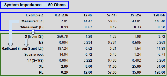
Numeric Examples

The table below shows $\vert Z_L \vert$ and $\vert \Gamma \vert$ for various load impedances, and then calculation of the load impedance using only those ‘measured’ quantities. It is not a mathematical proof, but does give examples to show that the eqation above works.

Visualiser

I wrote this visualiser to support this page, hosted on codepen. You can click and drag (or touch and drag) the load impedance point and see how the circles behave. Note that when the load is close to being purely resistive, any measurement errors resulting in a change to the relative radii of the two circles will produce a larger error in the load reactance than for load impedances away from the resistance axis. This seems to be a fundamental problem for this type of impedance measurement approach, tbc.

See the Pen ModZmodGamma by Alan (@DrAlan) on CodePen.